GitHub | GitLab mirror | Preprint

Examples¶

This page provides short, ready-to-run examples and selected visual outputs for the main CABS-flex standalone 3 workflows: protein flexibility, peptide modeling, and peptide–protein docking. For selected published applications focused on protein flexibility simulations and peptide-protein docking, see Published Applications.

1. Protein Flexibility¶

⬆ Back to top

1.1 Default simulation¶

To run CABS-flex using the default settings (see Modeling Workflow) use the following command:

CABSflex -i PDB/FILE

For example:

CABSflex -i 1hpw

This command downloads the 1hpw.pdb file from the PDB database and starts a simulation with default protein flexibility settings.

If the structure file is already available in the working directory, use:

CABSflex -i 1hpw.pdb

This command would try to open file 1hpw.pdb from working directory.

1.2 pLDDT-guided simulation¶

For AlphaFold models, pLDDT scores can be used to guide restraint generation and flexibility modeling. Regions with lower pLDDT values are treated as more flexible.

If pLDDT scores are stored in the B-factor column of the PDB file:

CABSflex -i model_af.pdb -g plddt --protein-plddt pdb

If the pLDDT scores are in a separate JSON file (from AlphaFold):

CABSflex -i model_af.pdb -g plddt --protein-plddt confidence.json

1.3 Protein Flexibility Visualizations¶

The following galleries showcase CABS-flex simulations for selected protein targets, grouped by PDB ID. Each section includes a brief description of the protein and selected visualizations of structural flexibility, such as RMSF heatmaps and worm-style ensemble views.

1C9S: Transcription attenuation protein MtrB¶

Transcription attenuation protein MtrB is a key regulator in Bacillus subtilis. The simulations capture the dynamic behavior of this protein, highlighting its structural flexibility and conformational sampling.

1BL8: Potassium channel KcsA¶

Potassium channel KcsA from Streptomyces lividans is a classic model for ion-channel studies. These visualizations show local fluctuations and flexible regions within its functional domains.

1EOV: Aspartyl-tRNA synthetase¶

Free aspartyl-tRNA synthetase (AspRS) from yeast differs from the tRNA-bound enzyme by structural changes in the catalytic site, hinge region, and anticodon-binding domain. These visualizations illustrate flexibility patterns in regions involved in conformational adaptation.

1GOY: Ribonuclease Bi¶

Ribonuclease Bi complexed with guanosine-3'-phosphate provides an example of enzyme flexibility near functional regions. The simulations illustrate local mobility around the active-site environment and complexed ligand.

1IJZ: Human IL-13¶

Human IL-13 is a cytokine involved in immune signaling and receptor interaction. The ensemble of models reflects flexible regions that may contribute to its biological function.

2. Peptide Modeling¶

⬆ Back to top

2.1 Linear peptide modeling¶

To predict the structure of a linear peptide from sequence, use:

CABSflex --peptide ACDEFGHIKLMNPQRSTVWY

2.2 Cyclic or constrained peptide modeling¶

To model a peptide with a distance restraint, for example between residues 2 and 8, use:

CABSflex --peptide ACDEFGHCKL --ca-rest-add 2:PEP 8:PEP 5.5 1.0

Distance restraints can be used to guide peptide sampling, including cyclic or otherwise constrained peptide conformations.

3. Peptide–Protein Docking¶

⬆ Back to top

3.1 Default Docking¶

To run CABS-dock using default settings, use:

CABSdock -i protein-pdb-code -p peptide-sequence:peptide-secondary-structure

For example, to dock the peptide HKLVQLLTTT with predicted secondary structure CHHHHHHHCC to chain A of PDB structure `2FVJ:

CABSdock -i 2FVJ:A -p HKLVQLLTTT:CHHHHHHHCC

This command:

• loads chain A from PDB structure 2FVJ as the receptor;
• defines the peptide sequence and secondary-structure assignment;
• runs docking with default settings;
• starts from random peptide positions and conformations;
• performs a broad search without prior knowledge of the binding site.

To extend the output with contact maps, configuration files, and simulation files, use:

CABSdock -i 2FVJ:A -p HKLVQLLTTT:CHHHHHHHCC -M -C -S

3.2 Global and local docking¶

CABS-dock can be used in both global and local docking settings.

In global docking, the peptide is sampled broadly around the receptor without prior information about the binding site. This mode is useful when the binding site is unknown or when the goal is to explore possible binding regions on the receptor surface.

In local docking, additional information can be used to restrict or guide the search toward a selected receptor region. This mode is useful when experimental data, structural knowledge, previous docking results, or predicted contacts suggest where the peptide should bind. The figure below compares sampling without contact information and with contact information for the 1LVM case. Without contact information, sampled peptide conformations are broadly distributed over the receptor surface. When contact information is provided, sampling is focused closer to the expected binding site, which can improve the selection of near-native models. The receptor residue used as contact information is highlighted in red; the experimental peptide is shown in magenta, global docking models in yellow, and information-driven docking models in cyan.

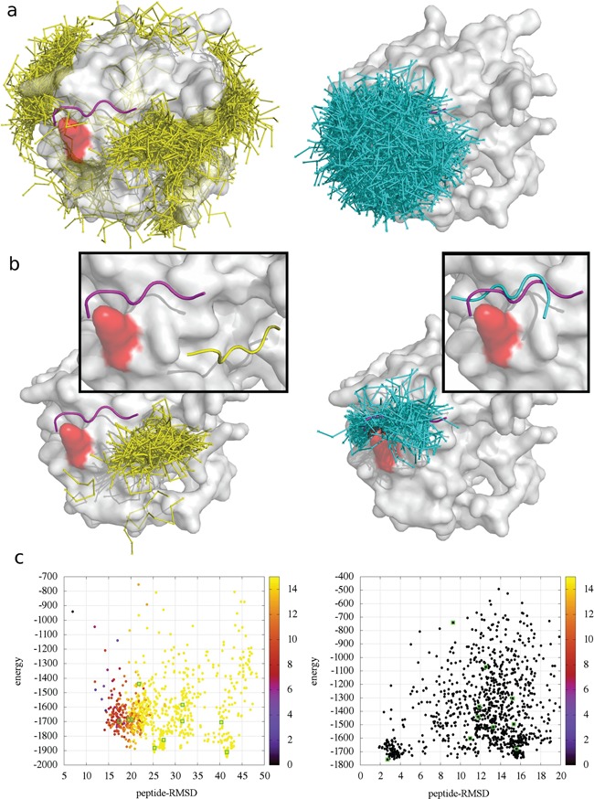
Figure. Global versus information-driven local docking in CABS-dock.

The examples below show local and global docking results for selected protein–peptide complexes.

1IHJ: N-terminal PDZ domain¶

The peptide is 5 amino acids long and adopts a beta-strand-like conformation.

1MVU: C219 monoclonal antibody scFv fragment¶

The Peptide is 13 amino acid long with helix secondary structure.

1KL3: Streptavidin complexed with strep-tag II peptide¶

This example shows docking of a short peptide to streptavidin.

3.3 Visualization of docking sampling: 1YCR case¶

This example visualizes a docking trajectory of the 15-residue p53-derived peptide SQETFSDLWKLLPEN to MDM2 (1YCR). The movie illustrates how a fully flexible peptide explores multiple positions, orientations, and conformations during the sampling stage. The simulations were performed using the following command. To increase sampling, the same setup was run three times using separate working directories (1ycr_r1, 1ycr_r2, and 1ycr_r3).

# Run 1; for additional independent runs, change r1 to r2 or r3
CABSdock -i 1ycr.pdb:A -p SQETFSDLWKLLPEN -R 1ycr.pdb:A:B -w 1ycr_r1 \
-a 20 -y 50 -s 200 -M -C -S -o A --renumber-residues-to-original \
--pdb-bfac-output A --csv-output A --json-output --dssp-output \
--ss-output --restraints-output --image-file-format svg --log \
--aa-rebuild T --aa-method cg2all --cg2all-representation calpha-sc \
--aa-rebuild-workers 24 --generate-chimera-visualizations \
--generate-pymol-visualizations --generate-notebook --aa-minimize

The energy-vs-RMSD plots below combine frames from three independent simulation runs. This gives a denser view of the sampled energy landscape than a single run would provide.

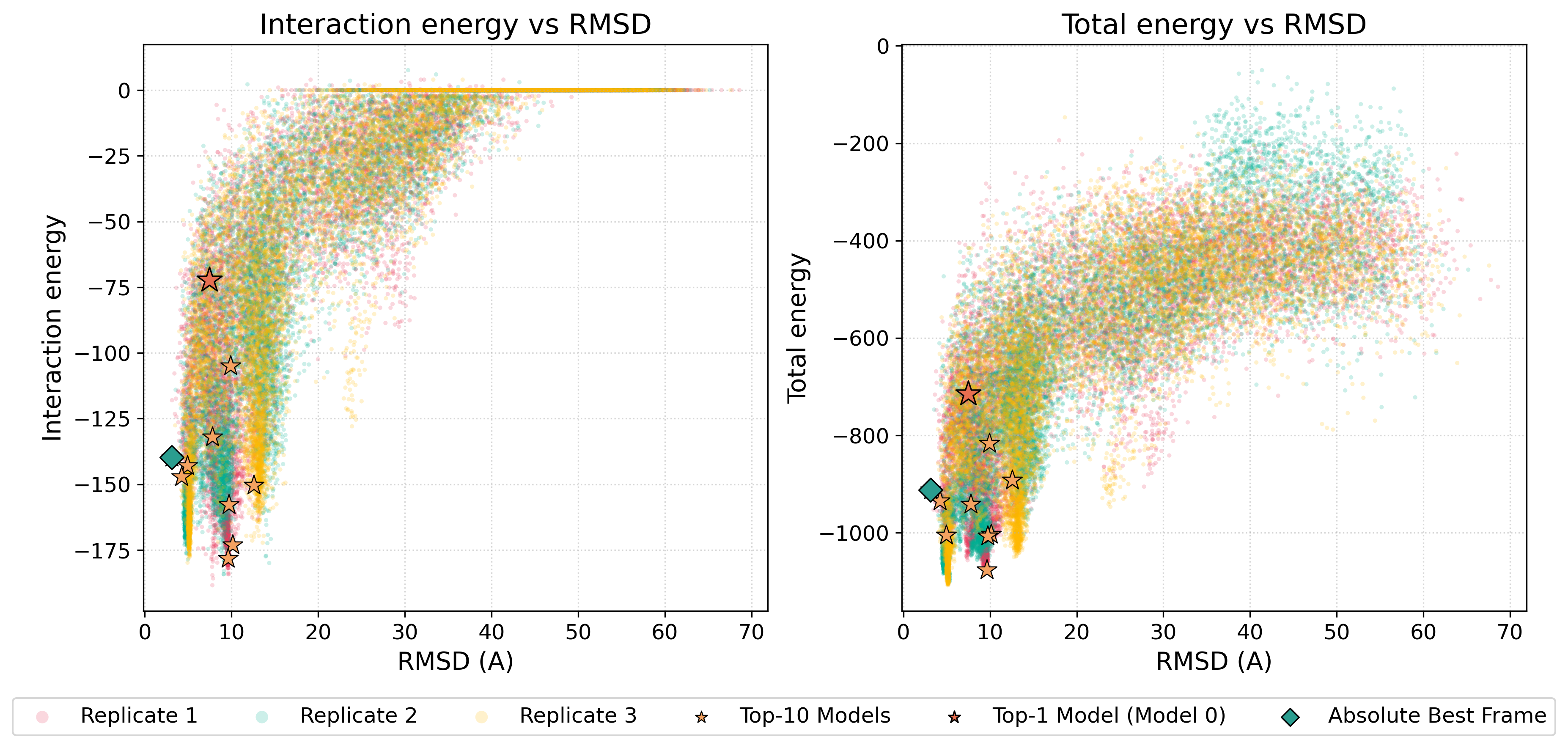
Figure. Energy-vs-RMSD plots for 1YCR. The panels show interaction energy and total energy plotted against RMSD for frames collected from three independent CABS-dock simulation runs. The top-ranked cluster medoids and the lowest-RMSD frame are highlighted.

Movie. Example of flexible peptide sampling in CABS-dock. This animation shows an example CABS-dock trajectory in which a fully flexible peptide explores multiple positions, orientations, and conformations around the receptor. Receptor flexibility is limited mainly to small backbone fluctuations and larger side-chain rearrangements. The movie illustrates the sampling stage used to search for possible binding modes before representative poses are selected.

Movie. Representative docking medoids. This rotating view shows the top 10 representative cluster medoids obtained from the docking simulation. Predicted peptide poses are shown together with the experimental reference peptide to illustrate the range of sampled binding poses selected after clustering.

← Peptide–Protein Docking | ⬆ Back to top | Next: Command-line Options