
![]() GitHub |
GitHub | ![]() GitLab mirror | Preprint
GitLab mirror | Preprint
Sampling and Temperature
Sampling
CABS simulations use Monte Carlo sampling to explore conformational space in the CABS coarse-grained representation. Instead of following atom-by-atom motions in real time, as in classical molecular dynamics, CABS generates trial conformational moves and accepts or rejects them according to an energy-based Metropolis criterion. As a result, CABS trajectories should be interpreted as pseudo-dynamic conformational ensembles, not as real-time MD trajectories.
This sampling scheme allows the model to efficiently explore both local fluctuations and larger cooperative motions of proteins and peptides. It is one of the key reasons why CABS-based workflows are useful for protein flexibility simulations, peptide modeling, and peptide–protein docking. For technical details of the CABS representation, force field, and Monte Carlo sampling scheme, see CABS reduced-representation model (Acta Biochimica Polonica 2004).
Simulation hierarchy
A CABS simulation is organized into three nested levels:
annealing cycles (-a)
└── MC cycles (-y) → one snapshot saved at the end of each MC cycle
   └── MC steps (-s)
The term annealing cycles comes from simulated annealing. In runs with identical initial and final temperatures, such as --temperature 1.4 1.4, these cycles should be understood simply as repeated sampling cycles.
One snapshot is saved at the end of each MC cycle, after the defined number of MC steps has been completed. Therefore, increasing -y increases the number of saved snapshots, while increasing -s extends the sampling between saved snapshots without increasing the number of output frames.
Main sampling parameters
| Parameter | Meaning |
|---|---|
-a, --mc-annealing |
number of annealing cycles |
-y, --mc-cycles |
number of MC cycles in each annealing cycle |
-s, --mc-steps |
number of Monte Carlo steps in each MC cycle |
For a single trajectory, the number of saved snapshots is:
A × Y
and the total number of Monte Carlo steps is:
A × Y × S
For example, with:
--a 20 --y 50 --s 50
the simulation produces:
20 × 50 = 1000 saved snapshots 20 × 50 × 50 = 50,000 MC steps
Replicas
Some workflows, especially peptide–protein docking, use multiple replicas.
A replica is an independent simulation run started from a different initial configuration or random seed. Replicas improve sampling by exploring several trajectories in parallel.
When replicas are used, the total number of saved snapshots becomes:
R × A × Y
and the total number of Monte Carlo steps becomes:
R × A × Y × S
For example, a docking setup with:
--replicas 10 --a 50 --y 50 --s 50
produces:
10 × 50 × 50 = 25,000 saved snapshots 10 × 50 × 50 × 50 = 1,250,000 MC steps
In practice:
| To do this | Change this |
|---|---|
| save more snapshots per trajectory | increase -y |
| make each trajectory longer between saved snapshots | increase -s |
| run more independent sampling attempts | increase --replicas |
| repeat more full sampling cycles | increase -a |
Interpreting CABS trajectories
CABS trajectories are useful for identifying flexible regions, comparing conformational states, generating representative models, and exploring possible large-scale motions. However, they should not be interpreted as exact physical trajectories with directly assigned real timescales.
The effective timescale of a CABS simulation is not defined a priori. It depends on the force field, temperature, restraints, system type, and simulation setup.
Temperature
The --temperature option controls how broadly the system explores conformational space during CABS sampling. In practical terms, it acts as a mobility control parameter: higher values allow broader motions and easier crossing of energetic barriers, while lower values keep the structure closer to the starting conformation or other low-energy states.
Although this parameter is called temperature, it is not expressed in Kelvins and cannot be directly converted to physical temperature units. It is a dimensionless reduced temperature used in the CABS Monte Carlo procedure.
What temperature does in practice
| Temperature setting | Typical effect |
|---|---|
| lower temperature | more conservative sampling, smaller fluctuations |
| higher temperature | broader sampling, larger fluctuations |
| decreasing temperature | broad exploration followed by more restrictive sampling |
The effect of temperature always depends on the full simulation setup, especially the restraint scheme. For example, the same temperature may produce moderate fluctuations with strong restraints, but very broad conformational sampling when automatic restraints are removed.
Constant temperature
If the initial and final temperature values are the same, the simulation runs at constant temperature.
Example:
--temperature 1.4 1.4
This is the default setting for many standard protein flexibility simulations. It provides a balance between conformational sampling and preservation of the overall fold.
Simulated annealing
If the initial and final temperature values differ, the simulation uses simulated annealing.
Example:
--temperature 2.0 1.0
In this setup, the simulation starts from a higher temperature, allowing broader exploration of conformational space, and then moves toward a lower temperature, making the sampling more restrictive.
This is useful in workflows where the search space is large, such as peptide–protein docking. At higher temperature, the peptide can explore different positions, orientations, and conformations. At lower temperature, the simulation becomes more focused on favorable binding poses.
Practical guidelines
Use the default temperature when:
- analyzing near-native protein flexibility,
- working with typical globular proteins,
- starting with a standard simulation setup.
Consider increasing the temperature when:
- broader conformational sampling is needed,
- studying disordered or highly flexible regions,
- exploring unfolding-like behavior,
- modeling peptides or highly mobile systems.
Use caution at higher temperatures, because excessive sampling may lead to structural distortion or ensembles that are harder to interpret.
Example: effect of temperature
The figure below illustrates the effect of temperature on CABS simulations of protein G (PDB ID: 2gb1) in the unleashed mode, where no automatic protein restraints are applied. As temperature increases, the RMSF profile becomes progressively higher and the conformational ensemble becomes broader. This example highlights the strong effect of temperature when sampling is driven primarily by the internal CABS force field.
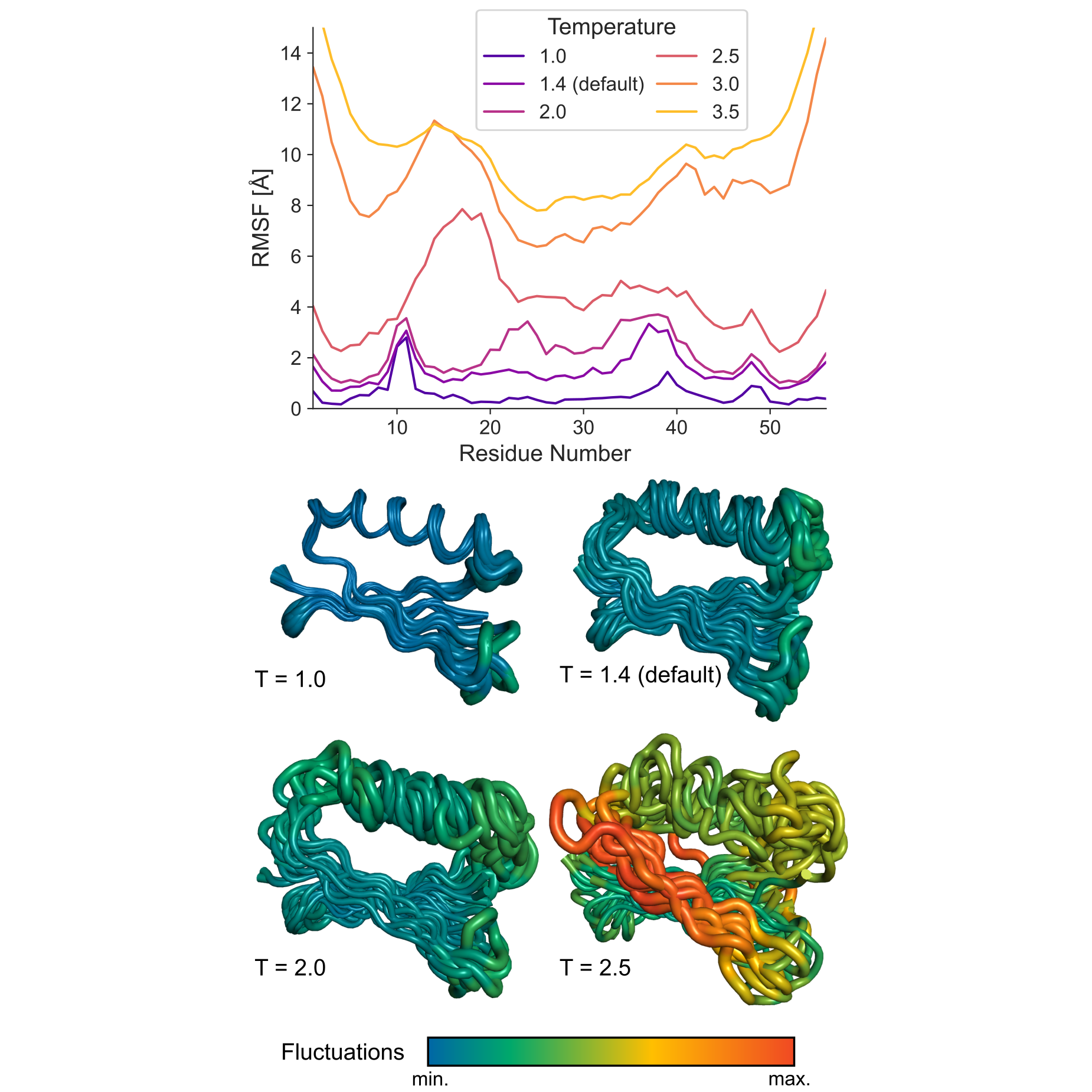
Figure. Effect of temperature on conformational sampling in CABS simulations. RMSF profiles and representative conformational ensembles obtained for protein G (PDB ID: 2gb1) at different CABS temperatures in the unleashed mode. Higher temperature values lead to broader sampling and larger fluctuations. The default temperature, T = 1.4, provides moderate flexibility, whereas higher values such as T = 2.0 or T = 2.5 produce substantially larger conformational variability.
← CABS Model | ⬆ Back to top | Next: Restraints